Vibe-training is our approach to building guardrails: instead of collecting labeled data and hand-tuning prompts, you describe the policy you want in plain language and get back a trained classifier. The “vibe” is the spec, and the pipeline turns it into a real fine-tuned model.
Our vibe-training platform ([platform link]) lets you train production-grade guardrails in a few minutes, and production-grade cuts along two axes: quality and performance. The first is about getting the classifier right. That’s the job of BARRED, the technique behind our training pipeline, which we covered in [previous blog post]. The second is getting that classifier to run in production, fast and at scale, which is what this post is about.
The two are tightly coupled. BARRED ships every guardrail as a LoRA adapter over a shared base model, and per-task adapters beat a one-size-fits-all judge on quality. But that design only pays off if you can actually serve those adapters under real load, and real load here is unforgiving.
Guardrails are blocking: nothing reaches the user until the relevant ones have run and passed, so a slow guardrail is a slow product. Our budget is sub-100ms p95. And they never come one at a time. A single application request typically fires 5 to 20 of them at once, each a different adapter, all due inside the same window.
So the problem this post tackles is serving a large, diverse population of LoRA adapters over a small base model, under bursty parallel load, without blowing the latency budget. Here’s how we did it.
We started off by studying the performance of our base model, without any LoRAs, to see where we land in terms of throughput for our latency budget.
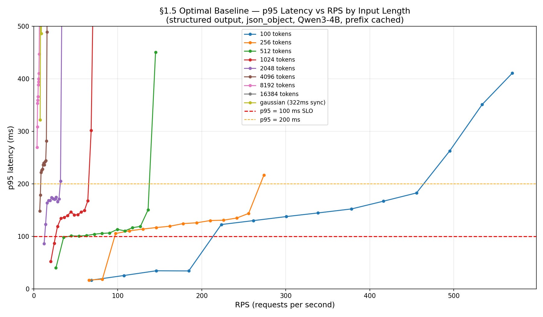
The basic shape of our workload is short requests (mostly < 4K tokens), structured output, and a single output token - i.e. prefill only.
We use a small base model (Qwen3-4B) on an H100 card.
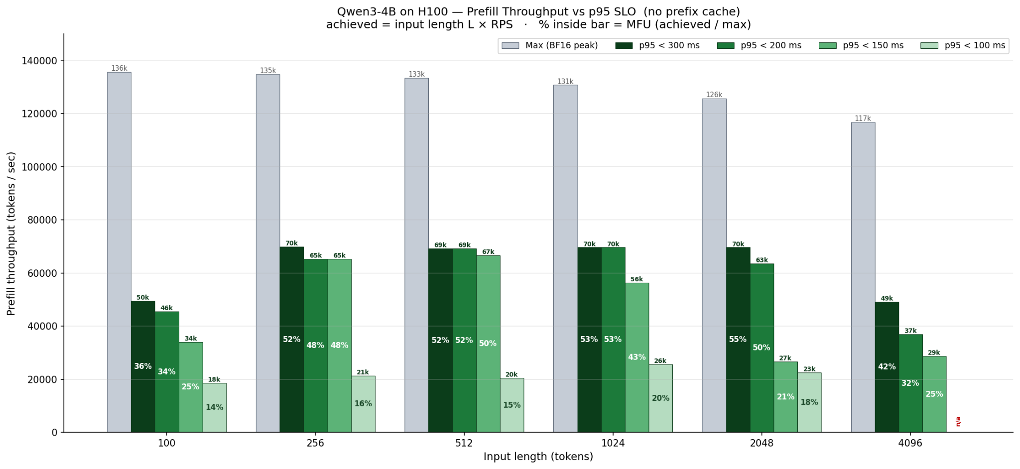
Utilizing this large card, capable of 989 TFLOPs/s would require us to do aggressive batching in each prefill step, to ensure the GEMM operations are saturated.
And here we encountered the first challenge: The target latency budget was p95 latency
of < 100 ms, which effectively leaves each scheduler step (batch) roughly 50ms net.
Since latency grows with batch size, we had to limit the number of tokens in a single batch, at a number which did not manage to saturate the hardware.
With too-small batches, we found that a fair amount of time was spent in the scheduler, launching kernels and generally overhead caused by frequent small batch launches.
To understand how well we were utilizing the GPU, we looked at our throughput in tokens/s and compared it to the maximal theoretical tokens/second that the GPU can achieve for our model.
The ratio between these two numbers is known as Model FLOPs utilization, or MFU.
As we can see, both very short inputs and longer inputs are finding short SLAs challenging.
The mid-sized inputs (256-2048) hit a more standard MFU of 50%, even in the face of our short SLA budget.
To keep batch sizes from growing and violating the SLA targets, we tuned the maximum batch size both in number of concurrent requests and total number of tokens to appropriate numbers.
We also tuned chunked prefills - which break down long prefill tasks down, and prefill them across multiple consecutive scheduler steps vs. have them dominate an entire step and starve shorter requests (thus leading to SLA violations).
Lastly, we did some tests to verify the effect of prefix caching, structured output overhead as well as the cost of additional output tokens to ensure we fully understood our performance envelope.
Still, our overall throughput and utilization from a single, expensive H100 node was not where we needed it to be - the machine still had plenty of headroom.
The solution was to serve multiple copies of the model on the same card.
vLLM doesn’t support running more than one copy of the model on the same GPU card under a single server process, so we had to roll out multiple servers, each with its own copy of the model (and KV cache…)
Naively starting two vLLMs on the same card doesn’t work well - even after you limit their memory fraction so that they can co-exist, the result is concurrency, not parallelism.
To achieve true parallelism, we considered two alternatives: MIG and MPS.
Given that our workload was high on overhead, we saw an opportunity to have the resource sharing be more collaborative than strict, thus allowing each process to make use of the full available resources on the card when it’s actually doing computation.
MPS sees batches originating from both vLLM as a single workload, which helps achieve real parallelism and real overlap in batch launches, which lead to higher GPU utilization and throughput.
We deployed two vLLM servers using MPS per H100 card, and saw a 50-100% improvement in our throughput without sacrificing latency, depending on the payload sizes.
So now, we had a way to deploy our base model and obtain high utilization, good throughput and keep our tight p95 SLA.
The next step was to introduce the main stars - our LoRA adapters.
In order to serve multiple LoRA adapters efficiently, we need to be able to execute batches of requests with heterogenous LoRA adapters per batch.
Batching together multiple LoRAs in a single forward pass is supported in vLLM using Punica kernels (implemented in Triton). These kernels allow to stack the LoRA weights, sort the batch by LoRA, and scan through the stack of LoRA weights in one kernel launch.
To make this kernel efficient, we wanted to use CUDA graphs. vLLM’s specialize-active-lora tells it to capture CUDA graphs for different numbers of active LoRAs per batch, thus ensuring that the actual computation is aligned with the actual batch shape.
Benchmarking showed us that the combination of these two capabilities (Punica kernels and specialize-active-loras) add a very small overhead to each batch in our system.
Before LoRA can participate in the batch, they have to be present in the GPU memory.
vLLM offers a multi-tier LRU caching system for LoRA weights, which can move LoRAs between the disk, the host (CPU) memory and the HBM.
At first, this seems like a big win - as it allows us to dynamically load and unload as many LoRA as we wanted, while we process batches, keeping the “hot” ones in GPU memory.
However, we quickly discovered that if even as few as 50% of the batch’s LoRAs have to be fetched from CPU, our SLA targets are breached.
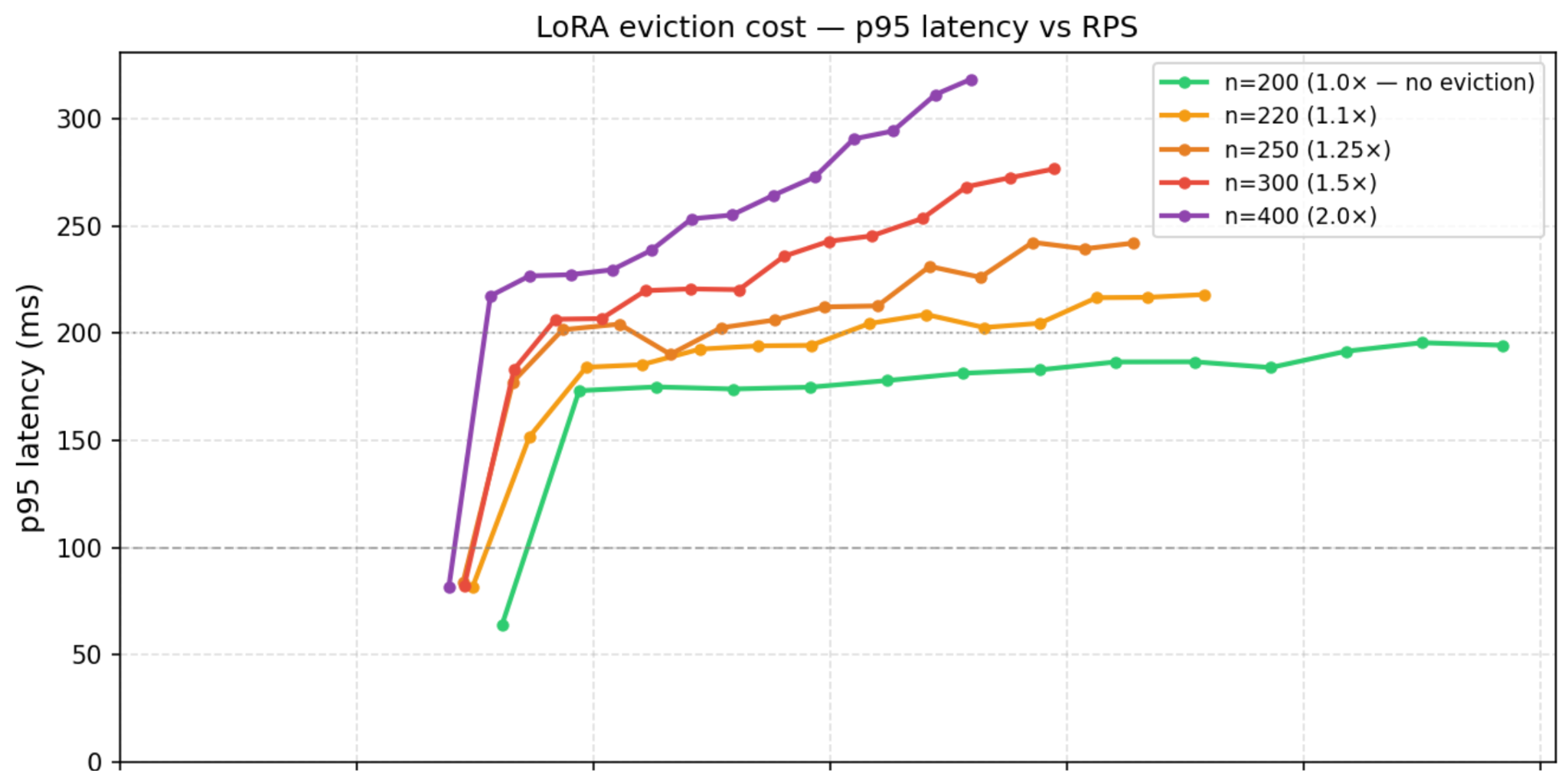
This is confirmed by paper analysis: each LoRA adapter weighs ~70MB, and fetching 10 of them over PCIe 4 would easily take 30-40 ms even from pinned memory.
As a result, we had to ensure all LoRAs were being served from GPU memory.
A quick back of the envelope calculation showed that between the model weights, the batch size, and the KV cache, an H100 node has room for roughly 400 LoRA adapters.
While 400 LoRAs per server is an impressive number, it is still only a fraction of our full LoRA repository.
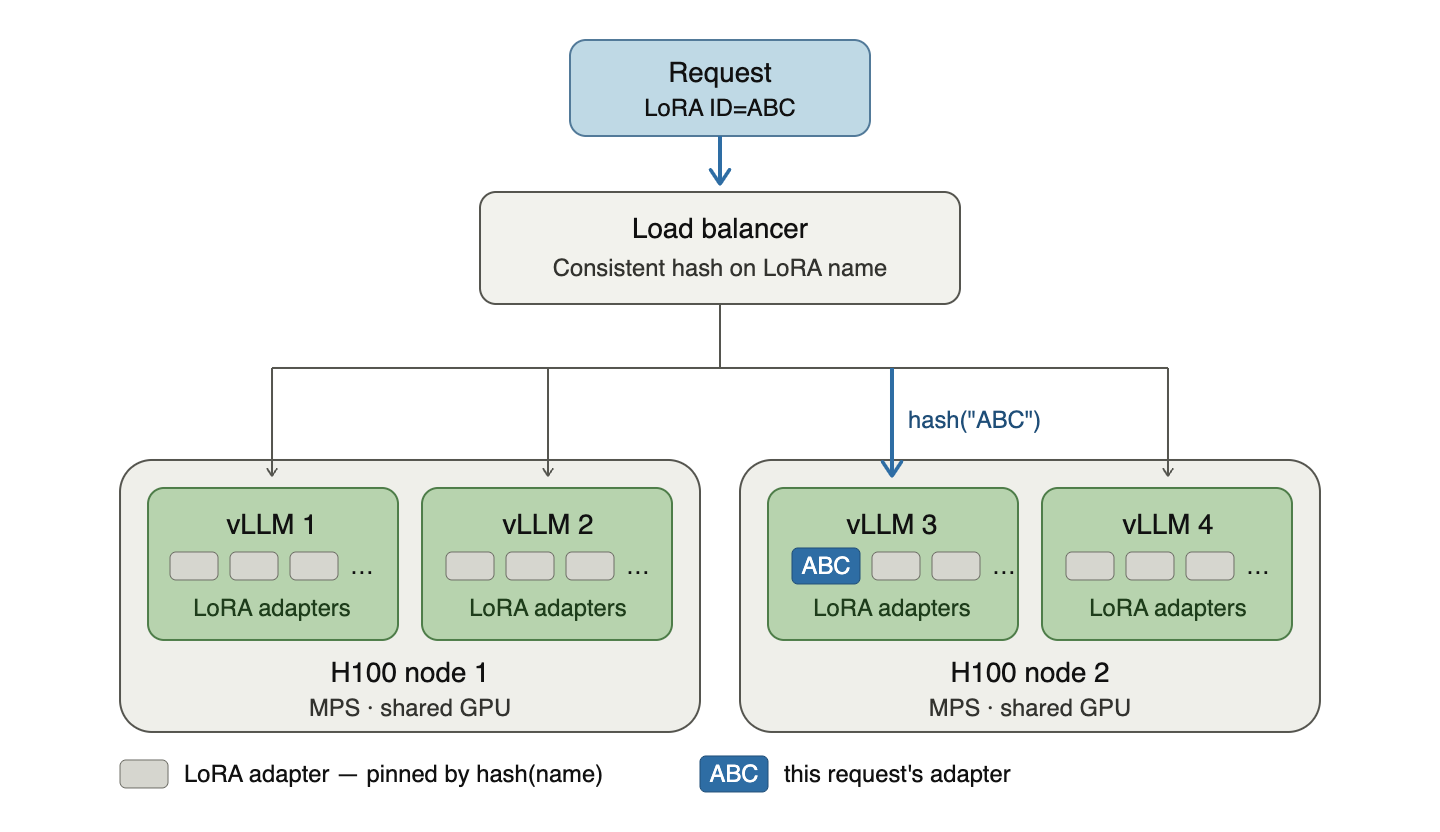
We had to find a way to spread the LoRAs across nodes.
Our solution was to load all LoRAs to CPU memory on all nodes, but then to load balance requests across servers using a consistent hash over the LoRA’s name.
This solution meant that different nodes would warm up different LoRAs, while adding new nodes would mean only a fraction of the LoRAs would need to migrate between nodes.
We set out to build a high throughput, low latency inference service which can handle thousands of LoRA adapters.
In order to saturate the GPU under a high-overhead workload of short inputs and small models, we deployed multiple vLLM instances on the same GPU using MPS, which led to a 50-100% increase in throughput while keeping our latency targets.
Serving thousands of LoRAs under strict SLA required careful use of vLLM’s LoRA-specific kernels. In addition, it required holding all LoRA adapters hot in GPU memory, which we achieved by load-balancing LoRAs across vLLM instances using consistent hashing routing.


.jpg)


.jpg)